N. GENGLER,![]() A. TIJANI,
A. TIJANI,![]() G. R.
WIGGANS,
G. R.
WIGGANS,![]() and I. MISZTAL
and I. MISZTAL![]()
*National Fund for Scientific Research, B-1000 Brussels,
Belgium![]() Animal Science Unit, Gembloux Agricultural University,
Animal Science Unit, Gembloux Agricultural University,
B-5030
Gembloux, Belgium![]() Animal Improvement Programs Laboratory, Agricultural
Animal Improvement Programs Laboratory, Agricultural
Research
Service, USDA, Beltsville, MD 20705-2350![]() Animal and Dairy Science
Department,
Animal and Dairy Science
Department,
University of Georgia, Athens 30605
Received December 15, 1998.
Accepted June 3,
1999.
1On leave from École Nationale
d'Agriculture, Meknès, Morocco.
1999 J. Dairy Sci.(Aug.)
Coefficients for (co)variance functions were obtained via random regression models using the expectation-maximization REML algorithm. Data included milk, fat, and protein yields from 176,495 test days of 22,943 first lactation Holstein cows that calved in Pennsylvania and Wisconsin from 1990 through 1996. Three approximately equal-sized data sets were created: one for Pennsylvania and two for Wisconsin. Random regressions were on third order Legendre polynomials. Genetic and permanent environmental (co)variances each were described by three coefficients. The model contained a fixed effect for age, season, and lactation stage rather than a fixed regression on days in milk. Fixed contemporary groups were based on herd, test day, and milking frequency. The coefficient matrices were dense and included approximately 70,000 equations. Estimated (co)variance function coefficients, as well as the heritabilities and correlations computed from them, were quite variable across data sets. Heritabilities were at a minimum (0.14 for milk and fat and 0.13 for protein) around peak yield, increased to a maximum (0.24 for milk and protein and 0.21 for fat) around the eighth month in milk, and declined slightly afterwards. Genetic correlations between early and late lactation were low (values of <0.10), especially for protein. Phenotypic correlations among test day yields were between 0.21 and 0.99.
[Key words: (co)variance function coefficients, test day model, heritability, correlation]
A (co)variance function can be defined as a continuous function that represents the variance and (co)variance of traits measured at different points on a trajectory (9, 10, 13). (Co)variance functions are particularly useful when spatial or temporal data are modeled, and a trajectory can be linked to phenomena that are space, age, or time dependent, such as growth or lactation. (Co)variance structures at any point along a continuous (time) scale can be predicted with (co)variance functions, and greater flexibility is possible in using measurements at any point along the trajectory. These functions allow information from all observations to contribute to each (co)variance.
For several years, the direct use of test day yields instead of computed or estimated 305-d lactation yields has been considered the next step in the evolution of genetic evaluation systems for dairy animals (e.g., 18, 28). Two types of test day models have been suggested: multitrait analysis proposed by Wiggans and Goddard (28) and random regression methods similar to those presented by Jamrozik et al. (5, 6). A challenge for both types of methods is to obtain correct variance components. Various studies have estimated those components (e.g., 2, 3, 4, 8, 12, 16, 17, 21, 26, 27), but in most cases few data or simplified models were used.
Full multitrait and random regression models are related. A full multitrait model might have each test day yield within a lactation as a distinct trait. In this case, (co)variance functions can be used to describe the full parameter space with a reduced number of parameters and to calculate (co)variances between any two traits. (Co)variance functions are equivalent to a regular multitrait (co)variance matrix of infinite dimension for which different traits are defined as points on the given trajectory (10). Random regression models, as proposed for test day models, developed historically from fixed regression repeatability models (18). These fixed regression models are still considered useful (19, 20) because of their relative simplicity. Random animal regression (23) was introduced next, and random permanent environmental regressions (22) were added later. Recently, the equivalence between random regression and multitrait models was shown (13, 25). This equivalence permits computation of (co)variance function coefficients directly as (co)variance components are estimated for the equivalent random regression model (11). The estimation of (co)variance components for random regression models has been described in several studies (4, 8, 22). Those studies show some potential difficulties, including wide variation in heritabilities and low correlations between early and late lactation.
The purpose of this study was to use expectation-maximization REML and random regression on polynomials to estimate (co)variance function coefficients for milk, fat, and protein test-day yields over the first 305 d of first lactation. A secondary objective was to compare the results with those reported earlier (3, 24) on similar data but using a multivariate method.
First lactation records of 22,943 Holstein cows were analyzed. Calvings occurred from 1990 through 1996 in 37 large herds in Pennsylvania and Wisconsin. Those two states were chosen because complete test day data were available and also because they represent two important dairy regions in the US. Initial data for test days consisted of milk yields as well as fat and protein percentages. Fat and protein yields were computed from milk yields and component percentages. A total of 176,495 test day records of first lactation cows between 7 and 305 DIM were used. The data were first subdivided by state. However, computation limitations made it necessary to subdivide further the Wisconsin data set. Herd identification numbers were used to create two approximately equal-sized files. Pedigree information was retrieved from the Animal Improvement Programs Laboratory database starting with cows with records. Ancestors born before 1981 were considered the base population. Eight genetic groups were assigned to unknown parents according to birth year (<1981, 1981 to 1982, 1983 to 1984, 1985 to 1986, 1987 to 1988, 1989 to 1990, 1991 to 1992, >1992). Tables 1 and 2 give additional information on the three subsets.
The model was designed to provide flexibility for the fixed portion and a minimum number of parameters for the random portion through the use of polynomials. To avoid imposing a particular form on the lactation curve, the curve was estimated as a series of fixed effects rather than as coefficients for a particular function. Random regression effects (genetic and permanent environment) and, therefore, (co)variances across test-days were modeled using Legendre polynomials to reduce correlations among regression coefficients. Third order polynomials (constant, linear, and quadratic) were used because preliminary research on (co)variance functions based on results of Tijani et al. (24) and Veerkamp and Goddard (27) showed that third order polynomials were sufficient for a single yield trait to describe the random variation around the fixed lactation curve. The polynomials were multiplied by 20.5, and, through this scaling, the constant regression coefficients became equivalent to the usual constant additive genetic effect. The three modified Legendre polynomials were
|
I0 = 1, |
|
I1 = 30.5x, and |
|
I2 = (5/4)0.5(3x2 - 1), |
where x = -1 + 2[(DIM - 1)/(305 - 1)].
The model was
y = Hh + Xb + Z*a + Zp + e,
where y = vector of test day milk, fat, or protein yields; h = vector of effects of classes for herd, test day, and milking frequency (two or three times daily); b = vector of effects of classes for age, season, and lactation stage; a = vector of genetic random regression coefficients (three per animal); p = vector of regression coefficients for permanent environment (three per cow with records); e = vector of residual effects; and H, X, Z, and Z* are incidence and covariate matrices where Z* is the covariate matrix Z augmented with columns for animals without records. Those matrices contained three columns per animal.
The following (co)variance structures were assumed:
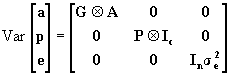
where G = (co)variance matrix for the genetic random
regressions [i.e., coefficients of the genetic (co)variance function], P
= (co)variance matrix for the permanent environmental random regressions [i.e.,
coefficients of the permanent environment (co)variance function], A =
additive genetic relationship matrix among animals,
Ic = identity matrix of dimension c (number of
cows or lactations),
![]() =
Kronecker product function, In = identity
matrix of dimension n (number of test day yields), and
=
Kronecker product function, In = identity
matrix of dimension n (number of test day yields), and
![]() =
residual variance.
=
residual variance.
Classes for age, season, and lactation stage were defined to avoid small classes. When using this model for routine genetic evaluation purposes, smaller classes would better account for these effects, but this precision was not deemed necessary for estimation of (co)variance functions. Classes for calving age were defined as 20 to 24, 25 to 26, 27 to 28, and 29 to 35 mo. Starting with January, six 2-mo calving seasons were defined. Twenty-two classes of lactation stage were defined: 7 to 13, 14 to 20, 21 to 27, 28 to 34, 35 to 41, 42 to 48, 49 to 55, 56 to 62, 63 to 76, 77 to 90, 91 to 104, 105 to 118, 119 to 132, 133 to 146, 147 to 167, 168 to 188, 189 to 209, 210 to 230, 231 to 251, 252 to 272, 273 to 293, and 294 to 305 DIM.
(Co)variance components were obtained using REMLF90 (14), which uses an expectation-maximization REML algorithm accelerated by the univariate Aitken extrapolation and sparse matrix modules in Fortran 90 including FSPAK90 (15). The modules make sparse matrix programming as efficient as if the functions were built into the programming language, and they are almost as easy to use as a matrix language. Additionally, the REMLF90 program was relatively simple compared with other REML programs and could be modified more easily. Computations were performed on a Digital Equipment Corporation (Marlboro, MA) Personal Workstation 433au (433 Mhz) with 512 MB of random access memory at the Gembloux Agricultural University computing center.
To test the goodness of fit of the proposed model, the residuals of the three data files were studied. Solutions for all effects in the model were obtained separately for all three data files using the (co)variance components estimated earlier. Computations were done on the same workstation as used for (co)variance components using a sparse matrix solver and Gauss-Seidel iterations to a convergence of relative squared solution below 10-10 or a maximum 300 iterations. Residuals were computed as the difference between the observed and the estimated values for a test day yield. Means and variances of residuals were computed by week of lactation.
Means and standard deviations of milk, fat, and protein yields are in Table 1. Milk, fat, and protein yields were lower in Pennsylvania than in Wisconsin, but yields generally were high in both states. Table 2 shows the numbers of animals included in the analyses. The three data sets included between 7173 and 8091 cows, and pedigree data included between 14,174 and 16,785 animals. The amount of data used in this study exceeded that of most other studies that have estimated variance components for random regression models (e.g., 4, 8), especially when models as complex as in this study were used.
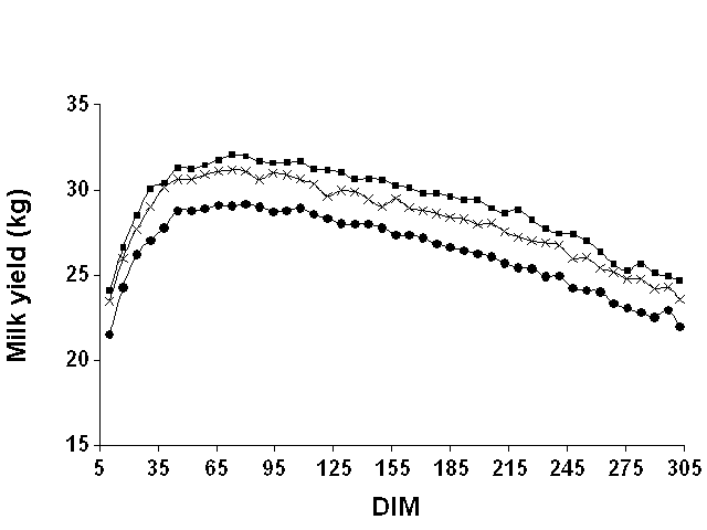
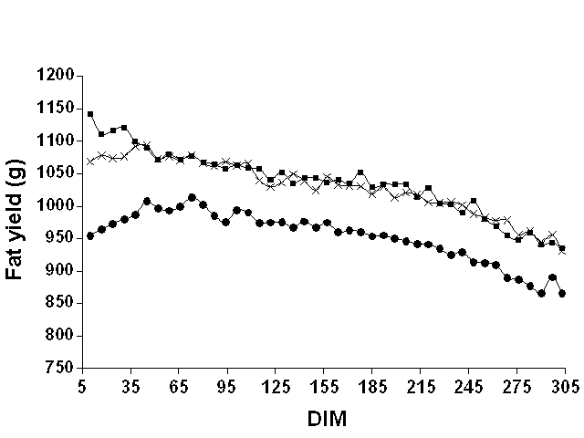
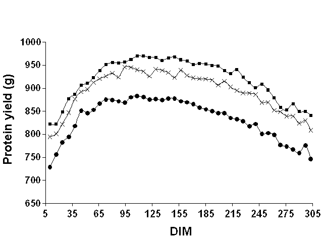
Figures 1, 2, and 3 show mean weekly milk, fat, and protein yields, respectively, over the lactation. For milk and protein, the curves were approximately parallel for the three data sets. For fat, the shape of the curve clearly differed between Pennsylvania and the two Wisconsin data sets. For Pennsylvania, fat yield tended to increase until around 65 DIM and then declined. However, for the Wisconsin data sets, fat yield decreased over the entire lactation. Milk yield peaked in both states around 65 DIM, whereas protein yield peaked later (between 100 and 150 DIM). These findings justified the use of DIM classes to model the mean of the lactation instead of imposing a particular function to represent a lactation curve.
|
Figure 1. Mean weekly test day milk
yields for Pennsylvania ( |
|
Figure 2. Mean weekly test day fat
yields for Pennsylvania ( |
|
Figure 3. Mean weekly test day protein
yields for Pennsylvania ( |
The numbers of equations for each data set also are in Table 2. The magnitude of the required computer processing is indicated by approximately 70,000 equations and inclusion of three genetic and three permanent environmental regressions in the models, which contribute to the density of the coefficient matrix. Variance component analysis of each data set required about 4 d of central processing unit time and required about 200 MB of memory. Estimation of solutions always required 300 Gauss-Seidel iterations and achieved convergences below 10-8.
Coefficients for genetic and permanent environmental (co)variance functions are in Tables 3 and 4, and estimates of residual variances are in Table 5. An interesting feature of the results was the variation in estimates for the same trait among data sets, which was found not only between but within region. Tables 3 and 4 also include the correlations among random regression coefficients. The genetic correlations (Table 3) showed a similar pattern across trait and sample. Constant genetic effect (I0) showed low to moderately high positive correlations with the linear (I1) and low to moderate negative correlations with the quadratic (I2) regression effect. Correlations between the linear (I1) and the quadratic (I2) regression effects were all moderately to strongly negative. Some differences existed among traits that could not be due only to sampling errors. Correlations (Table 4) among permanent environment effects showed, in general, values that were much closer to zero than for genetic effects. Also, patterns across samples and across traits were less similar; for example, some negative and positive values were obtained for the same correlations. But overall differences among samples by trait were rather small and probably due to sampling errors. Differences among traits were observed, especially between fat and protein in which two out of three correlations were in opposite directions. This study was unable to determine whether these differences were systematic.
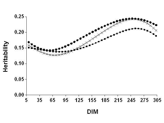
Heritabilities computed from (co)variance functions are in Table 6. The DIM are the midpoints of 12 25-d periods across lactation. Similar to the coefficients for (co)variance functions, heritability estimates were highly variable across subsets with extreme differences of up to 0.11. Genetic and total variances were computed from (co)variance functions at every DIM. Heritabilities were estimated as the ratio of genetic to total variance at every DIM. Mean heritability was obtained using mean coefficients for (co)variance functions (Figure 4). The heritability curves for all three yield traits showed an unexpected pattern. Heritabilities decreased to a minimum around 68 DIM, which corresponded to peak milk yield, then increased to a maximum around 243 DIM, and finally declined somewhat for the remainder of lactation. Results for the three data sets and yield traits (Table 6) showed similar patterns. A similar finding has been reported in at least two other studies (8, 22), which reported higher heritabilities for earliest stages than for peak yield. This result was difficult to explain even if different parts of the lactation curve were partly controlled by different genes. Peak production could have been less heritable because at peak some differences (e.g., the last additional kilograms produced) were more random and unpredictable than at lower levels of production.
|
Figure 4. Weekly estimates of
heritability computed from mean coefficients of (co)variance functions for milk
( |
The heritability findings could be an artifact of the type of model. However, Tijani et al. (24), who studied a similar data set using a slightly different approach, reported a similar pattern for milk and protein heritabilities except for the beginning of lactation. Tijani et al. (24) fit (co)variance functions on results from Gengler et al. (3), who estimated (co)variance components for a multitrait model similar to the one proposed by Wiggans and Goddard (28). The heritabilities estimated in this study were generally approximately 20% greater than those reported by Tijani et al. (24) but were still low compared with the estimates obtained with a similar model using Canadian data (20). The estimates from this study were similar to results of most other studies on heritability of test day yield (e.g., 8) that used random regression models. Results also were similar to those of Keown and Van Vleck (7) who found heritabilities of similar magnitude with maximum values about 2 mo earlier. This shift may reflect changes in production levels in the intervening 30 yr or could result from use of covariance functions.
Genetic and phenotypic correlations obtained from mean (co)variances among 12 evenly spaced test days between 18 and 293 DIM are in Table 7. Results for the three data sets (not shown) indicated some differences in correlations, especially between test days during early and late lactation for which genetic correlations were negative for some subsets. Mean phenotypic correlations were close to estimates from Tijani et al. (24). However, mean genetic correlations were different from those in that study (24) and were low, especially for correlations between test days during early and late lactation. Low correlations between early and late lactation were similar to those reported by Schaeffer (22) from a study using random regression models. The general tendency could have been that random regression models produced lower genetic correlations than did multitrait methods. In a similar comparison of random regression and multitrait models, Kettunen et al. (8) found correlations to be more similar but still lower for random regression.
Random regression models have the theoretical power to describe the (co)variance structure in a multivariate space in an infinite dimensional manner, which means that (co)variance estimates must fit into regression functions. However, (co)variances estimated through multitrait models can assume all values as long as the entire (co)variance matrix is positive definite and, therefore, have greater flexibility. A theoretical method to improve random regression models could be to identify other than genetic and permanent environmental sources of (co)variances between test day records of a cow and across cows such as autoregressive residuals or effects within and across lactation (e.g., 1), common calving seasons, and herd yield levels. Only Veerkamp and Goddard (27) have investigated the influence of herd yield levels using a (co)variance function approach. They found that heritabilities differed by herd yield level and that genetic correlations across herd yield levels and lactation stages could be rather small.
To determine the distribution of residuals (Table 8), means, standard deviations, minimum, and maximum were computed for milk, fat, and protein yield residuals. Compared with results in Table 1, standard deviations of residuals represented approximately 40 to 50% of standard deviations of original records.
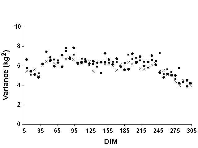
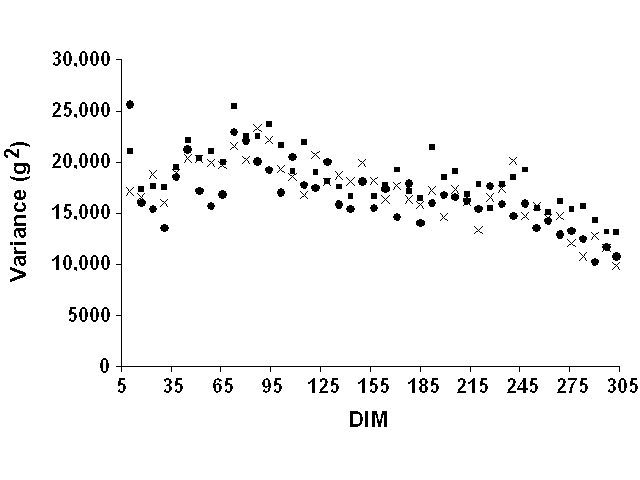
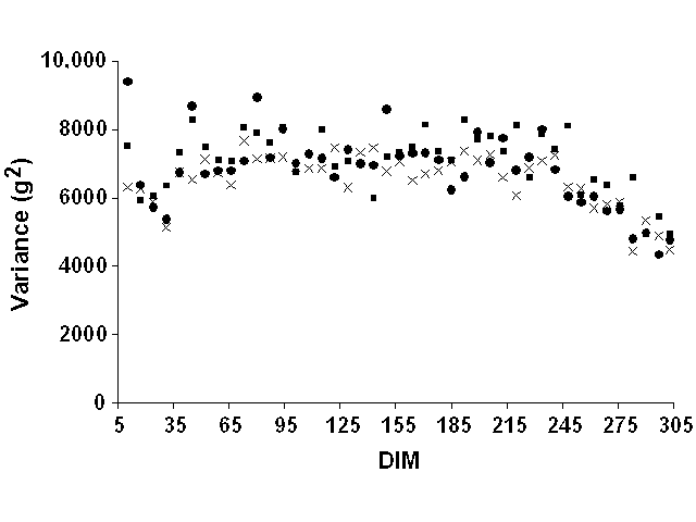
Weekly means were computed but were not very informative. Most mean deviations by week of lactation were zero because of the definition of lactation stages on a weekly basis. They were, therefore, not reported. For all yield traits and data sets, weekly variances of residuals tended to increase slightly at the beginning of lactation and to decrease slightly at the end (Figure 5 for milk yield, Figure 6 for fat yield, and Figure 7 for protein yield). However, definition of error variance as constant over the lactation still appeared to be justified. Therefore, variable error variances defined as linear and quadratic functions of DIM by Jamrozik et al. (6) would not be necessary. For a similar model, Schaeffer (22) reported a ratio of nearly 1 to 3 between the lowest and highest estimates of residual variance for milk yield. In this study, however, the residual variance displayed a nearly constant ratio (1:1.5) between lowest and highest variances after smoothing the residual variances for outliers that resulted from the limited number of records.
|
Figure 5. Weekly residual variances for
milk yield for Pennsylvania ( |
|
Figure 6. Weekly residual variances for
fat yield for Pennsylvania ( |
|
Figure 7. Weekly residual variances for
protein yield for Pennsylvania ( |
Analysis of residuals showed that the model chosen for this study fit the mean if lactation stages were short enough to adequately represent variations of yields over short periods. The model also accommodated the variance over the entire lactation. Use of this model instead of the model proposed by Jamrozik et al. (6) would avoid the necessity of adjusting residuals, thereby simplifying setting up the equations.
Coefficients for (co)variance functions can be obtained from random regression models with general expectation-maximization REML using a sparse matrix solver for models exceeding 70,000 relatively dense equations.
Estimates of (co)variance function coefficients showed large differences between data sets, which indicated substantial sampling errors. Those errors might be a major obstacle in the estimation of random regression (co)variance components and could explain the results in this study for heritabilities and (co)variances. Heritabilities declined to a minimum around peak yield, increased to a maximum around 245 DIM, and then declined slightly afterward. Genetic correlations were less than those estimated with nearly the same data using a multitrait model (3, 24), confirming a finding that was reported recently by other authors. Heritabilities were generally around 20% greater (estimates up to 0.25) than those reported in the studies involving similar data (3, 24).
The results show that further research on general comparison of models is needed as well as on alternative ways of modeling the mean and the (co)variances between test days. (Co)variance components estimated with random regression models may be seriously affected by numerical instability problems and by problems at the limits, especially the beginning of lactation (22). For multitrait models, the traditional way to improve numerical stability for highly correlated traits is through the use of canonical transformation. For random regression models, an internal canonical transformation could transform correlated regressions to uncorrelated regressions (25) and be used to stabilize estimation. The use of uncorrelated regressions would also eliminate the off-diagonal blocks linked to the (co)variances between regressions and would eliminate a part of the density of the coefficient matrix. An indirect benefit is that the amount of data that could be analyzed would increase, and, therefore, the sampling variance of the estimates would be reduced.
Nicolas Gengler, who is research team leader of the National Fund for Scientific Research, Brussels, Belgium, acknowledges its financial support. Aziz Tijani acknowledges the support of the General Administration of Development Cooperation, Brussels, Belgium. Ignacy Misztal acknowledges partial support from the Holstein Association. The authors thank J.H.J. van der Werf, University of New England, Armidale, Australia; R. F. Veerkamp, Institute for Animal Science and Health, Lelystad, The Netherlands; and J. C. Philpot and S. M. Hubbard, Animal Improvement Programs Laboratory, ARS, USDA, Beltsville, Maryland, for manuscript review.
REFERENCES |
|
| 1 |
Carvalheira, J.G.V., R. W. Blake, E. J. Pollak, R. L. Quaas, and C. V. Duran-Castro. 1998. Application of an autoregressive process to estimate genetic parameters and breeding values for daily milk yield in a tropical herd of Lucerna Cattle and in United States Holstein herds. J. Dairy Sci. 81:2738-2751. |
| 2 |
García-Cortés, L. A., C. Moreno, L. Varona, M. Rico, and J. Altarriba. 1995. (Co)variance component estimation of yield traits between different lactations using an animal model. Livest. Prod. Sci. 43:111-117. |
| 3 |
Gengler, N., A. Tijani, G. R. Wiggans, C. P. Van Tassell, and J. C. Philpot. 1999. Estimation of (co)variances of test day yields for first lactation Holsteins in the United States. J. Dairy Sci. 82:(Jan). Online. Accessed Jan. 11, 1999. |
| 4 |
Jamrozik, J., and L. R. Schaeffer. 1997. Estimates of genetic parameters for a test day model with random regression for yield traits of first lactation Holsteins. J. Dairy Sci. 80:762-770. |
| 5 |
Jamrozik, J., L. R. Schaeffer, and J.C.M. Dekkers. 1996. Random regression models for production traits in Canadian Holsteins. Pages 124-134 in Proc. Open Session INTERBULL Annu. Mtg., Veldhoven, The Netherlands, June 23-24, 1996. Int. Bull Eval. Serv. Bull. No. 14. Dep. Anim. Breed. Genet., Sveriges Lantbruks Universitet, Uppsala, Sweden. |
| 6 |
Jamrozik, J., L. R. Schaeffer, and J.C.M. Dekkers. 1997. Genetic evaluation of dairy cattle using test day yields and random regression model. J. Dairy Sci. 80:1217-1226. |
| 7 |
Keown, J. F., and L. D. Van Vleck. 1971. Selection on test day fat percentage and milk production. J. Dairy Sci. 54:199-203. |
| 8 |
Kettunen, A., E. A. Mäntysaari, and I. Strandén. 1997. Analysis of first lactation test day milk yields by random regression model. Pages 39-42 in Proc. Open Session INTERBULL Annu. Mtg., Vienna, Austria, Aug. 28-29, 1997. Int. Bull Eval. Serv. Bull. No. 16. Dep. Anim. Breed. Genet., Sveriges Lantbruks Universitet, Uppsala, Sweden. |
| 9 |
Kirkpatrick, M., W. G. Hill, and R. Thompson. 1994. Estimating the (co)variance structure of traits during growth and ageing, illustrated with lactation in dairy cattle. Genet. Res. Camb. 64:57-66. |
| 10 |
Kirkpatrick, M., D. Lofsvold, and M. Bulmer. 1990. Analysis of the inheritance, selection and evolution of growth trajectories. Genetics 124:979-993. |
| 11 |
Meyer, K. 1998. Modelling 'repeated' records: covariance functions and random regression models to analyse animal breeding data. Proc. 6th World Congr. Genet. Appl. Livest. Prod. 25:517-520. |
| 12 |
Meyer, K., H. -U. Graser, and K. Hammond. 1989. Estimates of genetic parameters for first lactation test day production of Australian Black and White cows. Livest. Prod. Sci. 21:177-199. |
| 13 |
Meyer, K., and W. G. Hill. 1997. Estimation of genetic and phenotypic (co)variance functions for longitudinal or "repeated" records by restricted maximum likelihood. Livest. Prod. Sci. 47:185-200. |
| 14 |
Misztal, I. 1998. REMLF90 manual. Mimeo, University of Georgia. ftp://num.ads.uga.edu/pub/blupf90/docs/remlf90.pdf. Accessed Nov. 27, 1998. |
| 15 |
Misztal, I., and M. Perez-Enciso. 1998. FSPAK90 - a Fortran 90 interface to sparse-matrix package FSPAK with dynamic memory allocation and sparse matrix structure. Proc. 6th World Congr. Genet. Appl. Livest. Prod. 27:467-468. |
| 16 |
Pander, B. L., W. G. Hill, and R. Thompson. 1992. Genetic parameters of test day records of British Holstein-Friesian heifers. Anim. Prod. 55:11-21. |
| 17 |
Pösö, J., E. A. Mäntysaari, and A. Kettunen. 1996. Estimation of genetic parameters of test day production in Finnish Ayrshire cows. Pages 45-48 in Proc. Open Session INTERBULL Annu. Mtg., Veldhoven, The Netherlands, June 23-24, 1996. Int. Bull Eval. Serv. Bull. No. 14. Dep. Anim. Breed. Genet., Sveriges Lantbruks Universitet, Uppsala, Sweden. |
|
Ptak, E., and L. R. Schaeffer. 1993. Use of test day yields for genetic evaluation of dairy sires and cows. Livest. Prod. Sci. 34: 23-34. |
|
| 19 |
Reents, R., J.C.M. Dekkers, and L. R. Schaeffer. 1995. Genetic evaluation for somatic cell score with a test day model for multiple lactations. J. Dairy Sci. 78:2858-2870. |
| 20 |
Reents, R., and L. Dopp. 1996. Genetic evaluation for dairy production traits with a test day model for multiple lactations. Pages 113-117 in Proc. Open Session INTERBULL Annu. Mtg., Veldhoven, The Netherlands, June 23-24, 1996. Int. Bull Eval. Serv. Bull. No. 14. Dep. Anim. Breed. Genet., Sveriges Lantbruks Universitet, Uppsala, Sweden. |
| 21 |
Rekaya, R., F. Béjar, M. J. Carabaño, and R. Alenda. 1995. Genetic parameters for test day measurements in Spanish Holstein-Friesian. Proc. Open Session INTERBULL Annu. Mtg., Prague, Czech Republic, Sept. 7-8, 1995. Int. Bull Eval. Serv. Bull. No. 11. Dep. Anim. Breed. Genet., Sveriges Lantbruks Universitet, Uppsala, Sweden. |
| 22 |
Schaeffer, L. R. 1997. Subject: random regressions. Anim. Breeders Discussion Group Log, Colorado State Univ. |
| 23 |
Schaeffer, L. R., and J.C.M. Dekkers. 1994. Random regression in animal models for test-day production in dairy cattle. Proc 5th World Congr. Genet. Appl. Livest. Prod. XVIII:443-446. |
| 24 |
Tijani, A., G. R. Wiggans, C. P. Van Tassell, J. C. Philpot, and N. Gengler. 1999. Use of (co)variance functions to describe (co)variances for test day yield. J. Dairy Sci. 82(Jan). Online. Accessed Jan. 11, 1999. |
| 25 |
van der Werf, J.H.J., M. E. Goddard, and K. Meyer. 1998. The use of covariance functions and random regressions for genetic evaluation of milk production based on test day records. J. Dairy Sci. 81:3300-3308. |
| 26 |
Vargas, B., E. Perez, and J.A.M. van Arendok. 1998. Analysis of test day yield data of Costa Rican dairy cattle. J. Dairy Sci. 81:255-263. |
| 27 |
Veerkamp, R. F., and M. E. Goddard. 1998. (Co)variance functions across herd production levels for test day records on milk, fat, and protein yield. J. Dairy Sci. 81:1690-1701. |
| 28 |
Wiggans, G. R., and M. E. Goddard. 1997. A computationally feasible test day model for genetic evaluation of yield traits in the United States. J. Dairy Sci. 80:1795-1800. |